Score centering (SC; Marek & Ryabinin, 2026) centers the training-policy score under the rollout policy. Let \(p\) and \(q\) be their next-token distributions at a sampled prefix, \(a\) the sampled token, and \(A\) its response’s detached GRPO advantage. We suppress response and token indices throughout. The unweighted, full-distribution SC loss is
Here \(\mathbb E_q\) includes rollout-group sampling, then averaging tokens within each response and responses within the group. The inner expectation is over the vocabulary at the fixed prefix. Training losses hold the rollout sampling law, probabilities, advantages and prefixes fixed; minibatch averages estimate these expectations. This is the original scalar loss, Appendix A.3, adapted to GRPO advantages and response normalization.
Why this centering works, where it remains biased, and how to repair that bias are the three questions below. The perspective was inspired by discussions with Jiacheng You.
1. Score centering: a change of perspective
The importance sampling approach
Rollouts come from \(q\), while the trainer evaluates \(p\). A familiar GRPO-style update multiplies the training score by a detached importance ratio:
Large ratios amplify sampling noise. TIS (Yao et al., 2025) uses the capped weight \(\min(\rho,c)\), with \(c=2\) here. TIS is one-sided truncation; GRPO instead uses PPO clipping with \(\epsilon=0.2\) in our experiments. This is a tokenwise surrogate with group advantages, not an exact full-response importance-sampling identity for expected reward. In multi-epoch GRPO, also distinguish the policy-version ratio \(p_{\mathrm{current}}/p_{\mathrm{old}}\) from the engine correction \(p_{\mathrm{old}}/q\); our fixed-checkpoint comparison has current = old.
The score centering approach
Instead, imagine that the rollout policy could backpropagate. Its GRPO-style reference update would be
This is the expected group-advantage update, rather than the raw expected-reward gradient. The inference engine supplies probabilities but usually no training backward pass. SC fills that gap using the trainer.
To see the mechanism, work with logits first. Let \(z_p\) produce \(p\) and let \(e\) be the one-hot vector of the sampled token. The derivative of log-softmax is \(e-p\). The derivative of its mean under detached \(q\) is \(q-p\). Subtracting gives
Centering replaces the trainer’s probability residual with the rollout policy’s residual. It still sends that residual through the training model’s backward pass.
This is precisely a straight-through estimator (Bengio et al., 2013): use the rollout logits in the forward pass and the training logits in the backward pass. With \(\operatorname{sg}\) denoting stop-gradient, construct
Forward evaluation sees \(z_q\), so log-softmax produces the same residual \(e-q\); backpropagation follows \(z_p\). The original SC loss and this STE loss have the same parameter gradient. Their scalar loss values differ.
| Method | Token weight | Forward / backward |
|---|---|---|
| IS | \(p/q\) | Training / training |
| TIS (\(c=2\)) | capped \(p/q\) | Training / training |
| SC as STE | 1 | Rollout / training |
| DRSC | 1 | Rollout / repaired training |
IS and TIS reweight a training-policy score. Unweighted SC approximates the rollout-policy update \(g_q\); DRSC improves that approximation. If the rollout checkpoint is stale, this reference is also delayed. It is not the exact gradient of today’s training objective. The original SC method can additionally be combined with IS; we study its unweighted form here.
2. Score centering is biased: how to fix it
2.1. Where the bias comes from
Now introduce the model Jacobians, \(J_p=\partial z_p/\partial\theta_p\) and \(J_q=\partial z_q/\partial\theta_q\). The chain rule turns the residual from Part 1 into a parameter update:
The probabilities and advantages agree; the backward maps do not. A different checkpoint can map the same logit residual to a different parameter direction. Matching forward probabilities alone therefore does not make SC unbiased.
Measured checkpoint mismatch. We use Qwen3.5-0.8B, all 752 million text parameters, and eight fixed SST-2 prompts. We restrict the next-token policy to A/B and renormalize over those two tokens. Four one-token responses form a group; enumerating its 16 ordered outcomes gives the exact expected update. The rollout checkpoint stays fixed while the CPU FP32 trainer takes four SGD updates (learning rate \(10^{-5}\)).
Figure 1 plots normalized squared bias, \(\|\mathbb E_q[\widehat g_B]-g_{\mathrm{ref}}\|^2/\|g_{\mathrm{ref}}\|^2\), averaged over prompts. Its left panel uses the rollout reference \(g_q\); the right uses the training reference \(g_p=\mathbb E_p[A\nabla_{\theta_p}\log p(a)]\), with groups and advantages recomputed under \(p\). Both use the same response/token averaging rule.
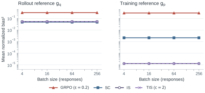
GRPO’s clipped update has a large bias under both references. IS and TIS have a visible gap to \(g_q\) but a much smaller bias to \(g_p\): some of that gap is a different target, not failed importance sampling. SC’s normalized bias² to \(g_q\) is 0.04922 at every batch size. The matched-weight controls give 0 for identical execution and \(8.98\times10^{-12}\) for chunk versus recurrent FP32 execution.
2.2. A better straight-through estimate via first-order approximation
For checkpoint lag, we know the displacement \(\Delta=\operatorname{sg}(\theta_q-\theta_p)\). Evaluate both checkpoints through the same smooth model implementation. A first-order Taylor expansion predicts the rollout logits:
SC uses only \(z_p\) as its backward proxy. Adding \(J_p\Delta\) captures how the logits changed as the checkpoint moved. Crucially, this term still depends on the training parameters. Differentiating with \(\Delta\) held fixed gives
Here \(H_z=\nabla^2_{\theta}z\) is the logit Hessian. Contracting one parameter axis with \(\Delta\) leaves a logit-by-parameter matrix, \(H_z(\theta_p)[\Delta]\), with the same shape as \(J_p\). This supplies the leading missing change in the backward map. We call the update derivative-repaired score centering (DRSC).
Theorem 1 (Local bias repair). Suppose both checkpoints use the same smooth logit map. Along the segment from \(\theta_p\) to \(\theta_q\), its Hessian has induced operator norm at most \(M\) and is Lipschitz with constant \(L\), uniformly over sampled prefixes. Set \(C=\mathbb E_q[\lvert A\rvert\,\lVert e-q\rVert]\), and keep \(\Delta\) detached. Then
Proof sketch. Taylor’s theorem gives
SC omits this entire term, whose norm is at most \(M\|\Delta\|\). DRSC includes \(H_z(\theta_p)[\Delta]\); Lipschitz continuity bounds the remaining integral by \(\int_0^1 Ls\|\Delta\|^2 ds=(L/2)\|\Delta\|^2\). Multiplying by \(A(e-q)\), taking expectations and applying the triangle inequality gives the bounds.
The repair changes first-order bias to second-order bias; squared bias changes from \(O(\|\Delta\|^2)\) to \(O(\|\Delta\|^4)\). In the Qwen test, normalized bias² falls from 0.005856 to 0.0000168 at one-update lag, and from 0.049218 to 0.001989 at four-update lag. These two checkpoints demonstrate a reduction, not an asymptotic scaling law.
The approximation is local. Studies of concentrated RL parameter changes (Mukherjee et al., 2025; Zhu et al., 2025) motivate examining checkpoint displacement, but retaining most delta energy or storing fewer parameters does not guarantee a small Taylor remainder.
2.3. Efficient implementation via JVP
The logit Hessian has a vocabulary axis and two parameter axes; materializing it is infeasible for an LLM. We only need its contraction in one checkpoint direction. A JVP computes \(J_p\Delta\) without constructing \(J_p\), and backpropagation through that result supplies the Hessian term. Keep the rollout logits as the forward value and the repaired proxy as the backward path:
The forward STE loss is unchanged. Only its backward proxy changes from \(z_p\) to \(z_p+J_p\Delta\).
Algorithm 1. Derivative-repaired score centering
- Collect rollout tokens, logits \(z_q\) and group advantages \(A\) from checkpoint \(\theta_q\); hold this batch fixed.
- Set \(\Delta\leftarrow\operatorname{sg}(\theta_q-\theta_p)\).
- Compute \((z_p,u)\leftarrow\operatorname{JVP}(z,\theta_p,\Delta)\), so \(u=J_p\Delta\).
- Form \(\widehat z_q\leftarrow z_p+u\) and \(\widetilde z^{\mathrm{DR}}\leftarrow\widehat z_q+\operatorname{sg}(z_q-\widehat z_q)\).
- Evaluate the DRSC loss on sampled tokens, averaging valid tokens per response and then responses.
- Backpropagate through both \(z_p\) and \(u\); update \(\theta_p\).
PyTorch’s torch.func.jvp computes \(J_p\Delta\) directly, without materializing a vocabulary-by-parameter Jacobian. Backpropagating through this JVP supplies the second-order term in the direction we actually need, rather than a full Hessian. Detach \(\Delta\), rollout logits and advantages, while keeping the JVP attached. Detaching the JVP removes the repair; differentiating the displacement cancels the base Jacobian term.
For rollouts sharing one checkpoint, the expected update can be written as a matrix-free Hessian-vector product (Pearlmutter, 1994):
Here \(A\) and \(e-q\) are detached: \(F\) is linear in logits, not a log-softmax loss. In code, replace the expectation with the response-normalized minibatch mean. Mixed rollout checkpoints use their own displacements and can be processed in checkpoint groups.
The correction adds trainer compute: our instrumented arithmetic test measured 34.3% more actor-training time, including diagnostics. In long-response LLM RL, rollout generation often dominates the cost (APRIL, 2025), so extra trainer work need not block rollout throughput when the trainer has spare capacity. The JVP cost should therefore be assessed against the pipeline bottleneck.
At identical master weights, \(\Delta=0\) and DRSC equals SC. This repair addresses checkpoint movement; it does not correct a mismatch caused purely by engine or precision differences.
3. Experiments
3.1. How good is the gradient estimate?
Goal: separate bias from sampling noise. Reuse the eight-prompt Qwen A/B setup above, with four-update checkpoint lag. The reference \(g_q\) uses the same group advantages (sample standard deviation, \(\epsilon=10^{-6}\)). Exact enumeration gives each estimator’s mean and variance; full-parameter VJPs and directional finite differences check the rollout reference.
For each prompt, divide all squared errors by \(\|g_q\|^2\), then average across prompts. Writing \(\mu_B=\mathbb E_q[\widehat g_B]\) and \(b_B=\mu_B-g_q\), the batch error decomposes as
\(B\) counts responses: \(B=4,16,64,256\) gives 1, 4, 16 or 64 independent groups per prompt. Averaging more groups reduces variance; the bias stays fixed.
Bias versus noise. Figure 2 shows MSE and variance separately. The reference remains \(g_q\), so IS and TIS include the target difference discussed above. We plot IS and TIS separately even though they coincide: the TIS cap \(c=2\) never activates here. GRPO uses PPO clipping with \(\epsilon=0.2\). The q-score oracle uses the rollout backward map and has zero bias to \(g_q\).
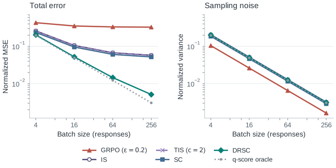
DRSC reduces SC’s squared bias by 96%, with about 8% more variance. At \(B=256\), MSE falls from 0.05213 to 0.00513. GRPO’s variance is smaller, but its bias² is 0.32527: clipping has discarded learning signal. More samples cannot recover that signal. Because these one-token responses share a prefix and their group advantages sum to zero, the common centering term cancels; this experiment isolates the backward-map repair.
Goal: isolate importance-weight noise. Reuse the constrained A/B policy, keep the master checkpoint fixed, and change rollout precision: native CPU BF16 autocast, or simulated INT4/INT3 weight rounding executed in FP32. For each setting, normalize variance by SC’s mean variance at \(B=4\) across the eight prompts. This denominator stays fixed as batch size grows:
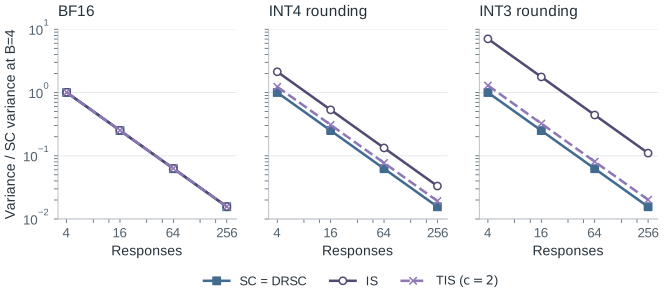
Every variance falls by 64 when moving from one to 64 independent groups. The relative gap remains: with INT3 rounding, IS needs about seven times as many samples to match SC’s variance; TIS caps most of that penalty. This precision test has no checkpoint displacement, so DRSC equals SC. It measures variance, not bias relative to a quantized-engine oracle, and does not benchmark native INT4/INT3 kernels.
3.2. Does it help actual RL training?
We train Qwen3.5-0.8B on \((a+b)\bmod10\) in SLIME, with Megatron-LM training and SGLang rollouts. Each run uses 30 Adam updates at learning rate \(10^{-6}\) and 16 prompts × four responses = 64 samples per update. All methods see the same 480 training questions, with operands in 0–99 and one-token answers. About 24% of responses are one update stale.
Seed 42 is a successful case; the correction does not consistently improve final accuracy across the four completed paired seeds.
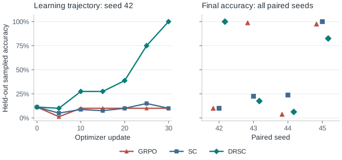
Evaluation samples four answers on each of 20 held-out questions. In seed 42 at update 30, GRPO always answers “1” and SC “3”; DRSC gets all 80 answers correct. The 64-response study has no TIS baseline.
GRPO applies PPO clipping, \(\epsilon=0.2\), directly to \(p/q\) with group-relative advantages. On the first stale mixed-reward group, the correct answer’s ratio is 0.000395: GRPO nearly removes its positive update, while clipping removes the three incorrect answers’ negative updates. SC and DRSC retain an unweighted signal. DRSC also reduces error to a behavior-checkpoint raw-score oracle on 25 of 29 inspected stale examples; this is a local score diagnostic, not a batch-gradient measurement.
These diagnostics do not establish the cause of SC’s collapse. DRSC outperforms SC only in seed 42 and underperforms it in the other three seeds; fresh seed-42 controls also collapse. The arithmetic run illustrates a successful case; the controlled gradient experiment directly establishes bias reduction.
3.3. Training and evaluation with 512 responses per update
A seed-42 follow-up uses 32 prompts × 16 responses = 512 samples in each optimizer update, with microbatch size 1 and gradient accumulation. It trains the same Qwen arithmetic task for 30 Adam updates at \(10^{-6}\), using 960 distinct training questions. This changes group size, questions and asynchronous settings as well as batch size; it is not a batch-size-only ablation of the earlier run.
The baseline here is TIS-GRPO: PPO clipping (\(\epsilon=0.2\)) uses the current/training-anchor ratio, with a separate detached engine weight \(\min(p_{\mathrm{anchor}}/q,2)\) applied once. This differs from the earlier direct-\(p/q\) GRPO baseline.
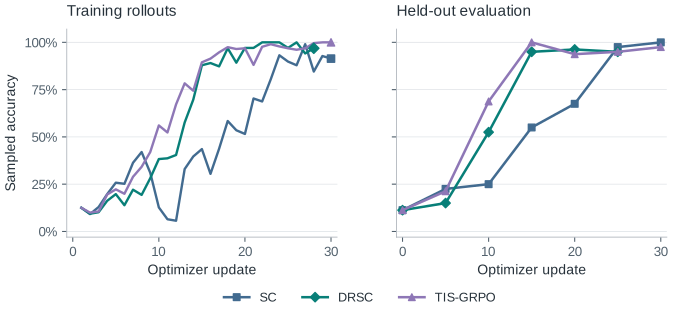
DRSC and TIS-GRPO reach high evaluation accuracy earlier than SC in this seed. SC reaches 100% at update 30 and TIS-GRPO 97.5%; DRSC’s latest evaluation is 95% at update 25. Its final evaluation is still unavailable in this snapshot. These are sampled accuracies from one seed and a small fixed test set.
4. Conclusion
SC uses the rollout residual with the trainer’s backward map. DRSC repairs its leading checkpoint error with one directional derivative, \(J_p\Delta\). The Qwen measurements show a lower bias floor, and the precision test isolates importance-weight noise. Whether this improved estimate gives reliable training gains remains open across the completed arithmetic seeds.
Reproducibility: download the data, estimator definitions and source hashes, checked October 12, 2026.